# matplotlib.use('Agg') # Removed to allow inline notebook plotting
import os
import psutil

# Set OMP_NUM_THREADS to avoid overhead on large machines
if "OMP_NUM_THREADS" not in os.environ:
    n_cores = psutil.cpu_count(logical=False)
    os.environ["OMP_NUM_THREADS"] = str(n_cores)
    print(f"OMP_NUM_THREADS set to {n_cores}")

from pysm3 import Sky
from pysm3 import units as u

import healpy as hp
import numpy as np
import matplotlib.pyplot as plt
import matplotlib.image as mpimg
from astropy.table import Table
from pysm3.models.websky import y2uK_CMB

OMP_NUM_THREADS set to 128

import logging
logging.getLogger("pysm3").setLevel(logging.INFO)

def remove_monopole(m):
    mono = np.mean(m)
    return m - mono, mono

def joint_limits(map_dict, percentile=99.5):
    stacked = np.concatenate([m.value.ravel() for m in map_dict.values()])
    vmax = np.percentile(np.abs(stacked), percentile)
    if vmax <= 0:
        vmax = np.max(np.abs(stacked))
    if vmax == 0:
        vmax = 1.0
    vmax = float(f"{vmax:.2g}")
    return -vmax, vmax

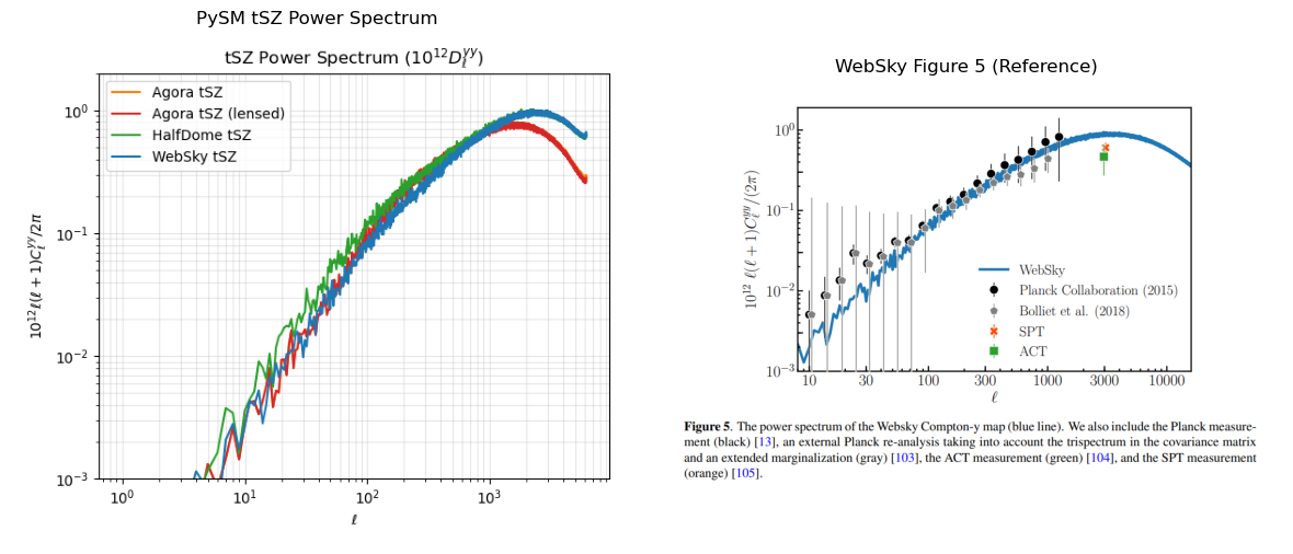
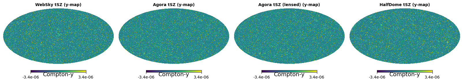
SZ realization comparisons

Summary plots and statistics for the thermal and kinematic SZ components.

models = ["tsz1", "tsz2", "tsz3", "tsz4"]
model_titles = {
    "tsz1": "WebSky tSZ",
    "tsz2": "Agora tSZ",
    "tsz3": "Agora tSZ (lensed)",
    "tsz4": "HalfDome tSZ",
}

skys = {model: Sky(nside=2048, preset_strings=[model], output_unit=u.uK_CMB) for model in models}

freq_ghz = 143
maps = {}
for model in models:
    cache_file = f"data/cache_tsz_{model}_{freq_ghz}GHz.fits"
    if os.path.exists(cache_file):
        print(f"Loading {model} tSZ from cache: {cache_file}")
        maps[model] = hp.read_map(cache_file, verbose=False) * u.dimensionless_unscaled
    else:
        print(f"Computing {model} tSZ at {freq_ghz} GHz...")
        maps[model] = skys[model].get_emission(freq_ghz * u.GHz)[0] / y2uK_CMB(freq_ghz)
        hp.write_map(cache_file, maps[model].value, overwrite=True)

Loading tsz1 tSZ from cache: data/cache_tsz_tsz1_143GHz.fits

/tmp/ipykernel_1558934/795449475.py:17: HealpyDeprecationWarning: "verbose" was deprecated in version 1.15.0 and will be removed in a future version.
  maps[model] = hp.read_map(cache_file, verbose=False) * u.dimensionless_unscaled

Loading tsz2 tSZ from cache: data/cache_tsz_tsz2_143GHz.fits
Loading tsz3 tSZ from cache: data/cache_tsz_tsz3_143GHz.fits
Loading tsz4 tSZ from cache: data/cache_tsz_tsz4_143GHz.fits

n_rows = 1
n_cols = len(models)
fig = plt.figure(figsize=(4.0 * n_cols, 4.2 * n_rows))
monopoles = {}

# Compute joint limits across all models in Compton-y
stacked = np.concatenate([maps[model].value.ravel() for model in models])
vmax = np.percentile(np.abs(stacked), 95)
if vmax <= 0:
    vmax = np.max(np.abs(stacked))
if vmax == 0:
    vmax = 1.0
vmax = float(f"{vmax:.2g}")
vmin = -vmax

for col_idx, model in enumerate(models, start=1):
    component = maps[model]
    centered_map, mono = remove_monopole(component)
    monopoles[model] = mono
    hp.mollview(
        centered_map,
        sub=(n_rows, n_cols, col_idx),
        fig=fig,
        min=vmin,
        max=vmax,
        unit="Compton-y",
        title="",
    )
    ax = plt.gca()
    ax.text(
        0.5,
        1.03,
        f"{model_titles[model]} (y-map)",
        transform=ax.transAxes,
        ha="center",
        va="bottom",
        fontsize=10,
        fontweight="bold",
    )

plt.subplots_adjust(hspace=0.45, top=0.88)

print("Monopoles removed (Compton-y):")
for model in models:
    print(f"  {model_titles[model]}: {monopoles[model]:.3e}")

Monopoles removed (Compton-y):
  WebSky tSZ: 1.238e-06
  Agora tSZ: 2.053e-06
  Agora tSZ (lensed): 2.053e-06
  HalfDome tSZ: 1.031e-06

diff = maps["tsz3"] - maps["tsz2"]
diff_data = diff.value
vmax = np.percentile(np.abs(diff_data), 99.5)
if vmax <= 0:
    vmax = np.max(np.abs(diff_data))
if vmax == 0:
    vmax = 1.0
vmax = float(f"{vmax:.2g}")
hp.mollview(
    diff_data,
    fig=plt.figure(figsize=(6, 4)),
    min=-vmax,
    max=vmax,
    unit="Compton-y",
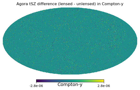
    title=f"Agora tSZ difference (lensed - unlensed) in Compton-y",
)
diff_stats = {
    "mean": float(np.mean(diff_data)),
    "rms": float(np.sqrt(np.mean(diff_data**2))),
    "p99": float(np.percentile(np.abs(diff_data), 99.0)),
}

print(f"Summary of tsz3 - tsz2 differences in Compton-y:")
print(
    f"  mean: {diff_stats['mean']:.3e}, rms: {diff_stats['rms']:.3e}, |diff|_99%: {diff_stats['p99']:.3e}"
)

Summary of tsz3 - tsz2 differences in Compton-y:
  mean: 1.893e-11, rms: 5.406e-07, |diff|_99%: 1.964e-06

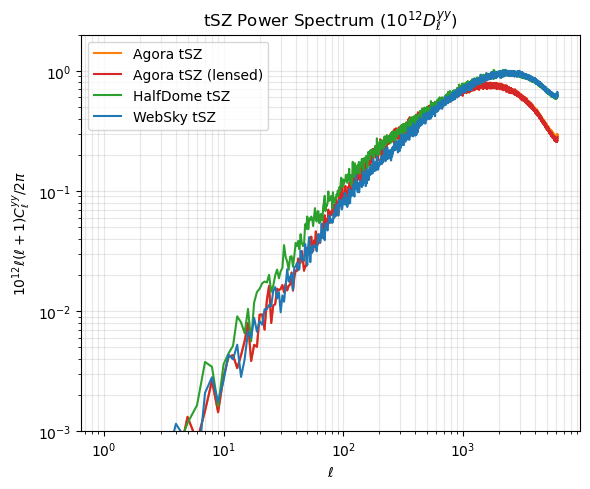
Reference: WebSky Figure 5 (tSZ)

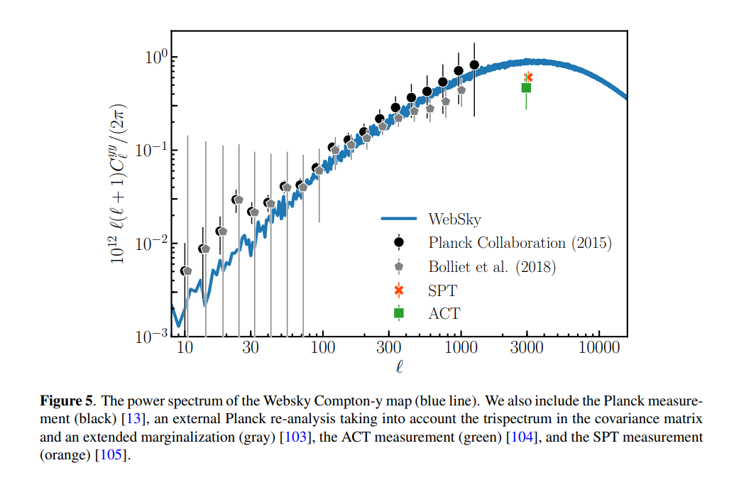
Comparison note: The plot below shows the Compton-y power spectrum in log-log scale.

lmax = 3 * 2048 - 1
ells = np.arange(lmax + 1)
d_ell_factor = ells * (ells + 1) / (2 * np.pi)

color_options = [
    "tab:red",
    "tab:purple",
    "tab:green",
    "tab:blue",
    "tab:orange",
]
model_colors = {
    "tsz1": "tab:blue",
    "tsz2": "tab:orange",
    "tsz3": "tab:red",
    "tsz4": "tab:green",
}

fig, ax = plt.subplots(figsize=(6, 5))
# Plot tsz1 (WebSky) last to ensure it is on top
for model in (models[1:] + [models[0]]):
    cls = hp.anafast(maps[model].value, lmax=lmax)
    # Dimensionless y-spectrum * 10^12
    d_ell_12 = d_ell_factor * cls * 1e12
    ax.loglog(ells[1:], d_ell_12[1:], color=model_colors[model], label=model_titles[model])

ax.set_title(f"tSZ Power Spectrum ($10^{{12}} D_\\ell^{{yy}}$)")
ax.set_xlabel("$\\ell$")
ax.set_ylabel("$10^{12} \\ell(\\ell+1)C_\\ell^{yy} / 2\\pi$")
ax.grid(True, which="both", alpha=0.3)
ax.legend(loc="upper left")
ax.set_ylim(1e-3, 2.0)
fig.tight_layout()
fig.savefig("tsz_power_spectrum.png")

# Kinematic SZ Comparisons
ksz_models = ["ksz1", "ksz2", "ksz3"]
ksz_titles = {
    "ksz1": "WebSky kSZ",
    "ksz2": "Agora kSZ",
    "ksz3": "Agora kSZ (lensed)",
}
ksz_freq = 143
ksz_skys = {model: Sky(nside=2048, preset_strings=[model], output_unit=u.uK_CMB) for model in ksz_models}
ksz_maps = {}
for model in ksz_models:
    cache_file = f"data/cache_ksz_{model}_{ksz_freq}GHz.fits"
    if os.path.exists(cache_file):
        print(f"Loading {model} kSZ from cache: {cache_file}")
        ksz_maps[model] = hp.read_map(cache_file, field=(0, 1, 2), verbose=False) * u.uK_CMB
    else:
        print(f"Computing {model} kSZ at {ksz_freq} GHz...")
        ksz_maps[model] = ksz_skys[model].get_emission(ksz_freq * u.GHz)
        hp.write_map(cache_file, ksz_maps[model].to_value(u.uK_CMB), overwrite=True)
ksz_colors = {
    "ksz1": "tab:gray",
    "ksz2": "tab:orange",
    "ksz3": "tab:red",
}
ksz_unit = str(next(iter(ksz_maps.values()))[0].unit)
print(
    f"Loaded kSZ templates at {ksz_freq} GHz (units: {ksz_unit}) -> "
    + ", ".join(ksz_titles[model] for model in ksz_models)
)

Loading ksz1 kSZ from cache: data/cache_ksz_ksz1_143GHz.fits

/tmp/ipykernel_1558934/165830930.py:15: HealpyDeprecationWarning: "verbose" was deprecated in version 1.15.0 and will be removed in a future version.
  ksz_maps[model] = hp.read_map(cache_file, field=(0, 1, 2), verbose=False) * u.uK_CMB

Loading ksz2 kSZ from cache: data/cache_ksz_ksz2_143GHz.fits
Loading ksz3 kSZ from cache: data/cache_ksz_ksz3_143GHz.fits
Loaded kSZ templates at 143 GHz (units: uK_CMB) -> WebSky kSZ, Agora kSZ, Agora kSZ (lensed)

fig = plt.figure(figsize=(4.0 * len(ksz_models), 4.0))
stacked = np.concatenate([ksz_maps[model][0].value.ravel() for model in ksz_models])
vmax = np.percentile(np.abs(stacked), 99.5)
if vmax <= 0:
    vmax = np.max(np.abs(stacked))
if vmax == 0:
    vmax = 1.0
vmax = float(f"{vmax:.2g}")
vmin = -vmax
ksz_monopoles = {}
for col_idx, model in enumerate(ksz_models, start=1):
    component = ksz_maps[model][0]
    centered_map, mono = remove_monopole(component)
    ksz_monopoles[model] = mono
    hp.mollview(
        centered_map,
        sub=(1, len(ksz_models), col_idx),
        fig=fig,
        min=vmin,
        max=vmax,
        unit=str(component.unit),
        title="",
    )
    ax = plt.gca()
    ax.text(
        0.5,
        1.03,
        f"{ksz_titles[model]} @ {ksz_freq} GHz",
        transform=ax.transAxes,
        ha="center",
        va="bottom",
        fontsize=10,
        fontweight="bold",
    )

plt.subplots_adjust(top=0.85, wspace=0.25)

print("kSZ monopoles removed (units in", ksz_unit, "):")
for model in ksz_models:
    print(f"  {ksz_titles[model]}: {ksz_monopoles[model]:.3e}")

kSZ monopoles removed (units in uK_CMB ):
  WebSky kSZ: -1.866e-01 uK_CMB
  Agora kSZ: 4.191e-02 uK_CMB
  Agora kSZ (lensed): 4.148e-02 uK_CMB

ksz_diff = ksz_maps["ksz3"][0] - ksz_maps["ksz2"][0]
ksz_diff_data = ksz_diff.value
vmax = np.percentile(np.abs(ksz_diff_data), 99.5)
if vmax <= 0:
    vmax = np.max(np.abs(ksz_diff_data))
if vmax == 0:
    vmax = 1.0
vmax = float(f"{vmax:.2g}")

fig = plt.figure(figsize=(6, 3.6))
hp.mollview(
    ksz_diff_data,
    sub=(1, 1, 1),
    fig=fig,
    min=-vmax,
    max=vmax,
    unit=str(ksz_diff.unit),
    title=f"kSZ difference ({ksz_titles['ksz3']} - {ksz_titles['ksz2']}) @ {ksz_freq} GHz",
)

ksz_23_stats = {
    "mean": float(np.mean(ksz_diff_data)),
    "rms": float(np.sqrt(np.mean(ksz_diff_data**2))),
    "p99": float(np.percentile(np.abs(ksz_diff_data), 99.0)),
}

print(
    "Summary of kSZ differences at",
    ksz_freq,
    "GHz (units in",
    str(ksz_diff.unit),
    "):",
)
print(
    f"  {ksz_titles['ksz3']} - {ksz_titles['ksz2']} -> mean: {ksz_23_stats['mean']:.3e}, rms: {ksz_23_stats['rms']:.3e}, |diff|_99%: {ksz_23_stats['p99']:.3e}",
)

Summary of kSZ differences at 143 GHz (units in uK_CMB ):
  Agora kSZ (lensed) - Agora kSZ -> mean: -4.237e-04, rms: 6.996e-01, |diff|_99%: 2.451e+00

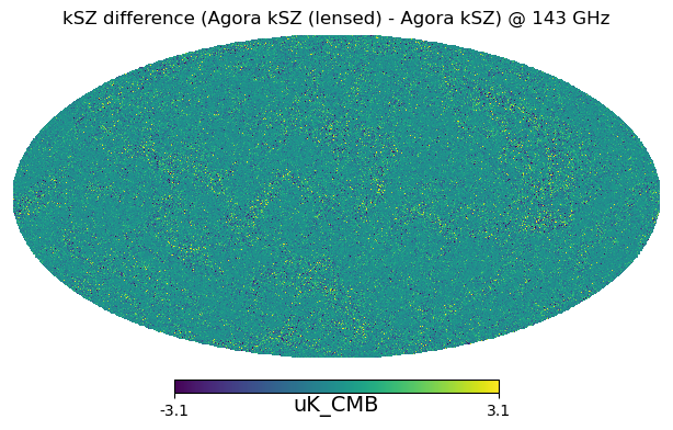
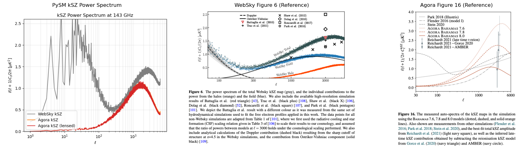
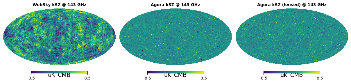
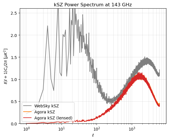
Reference: WebSky Figure 6 (kSZ)

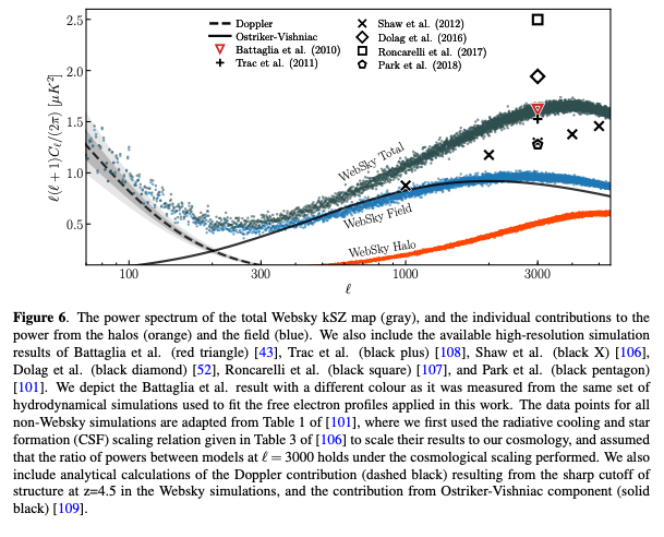
Comparison note: The kSZ power spectrum is plotted in semilogx with units of uK^2.

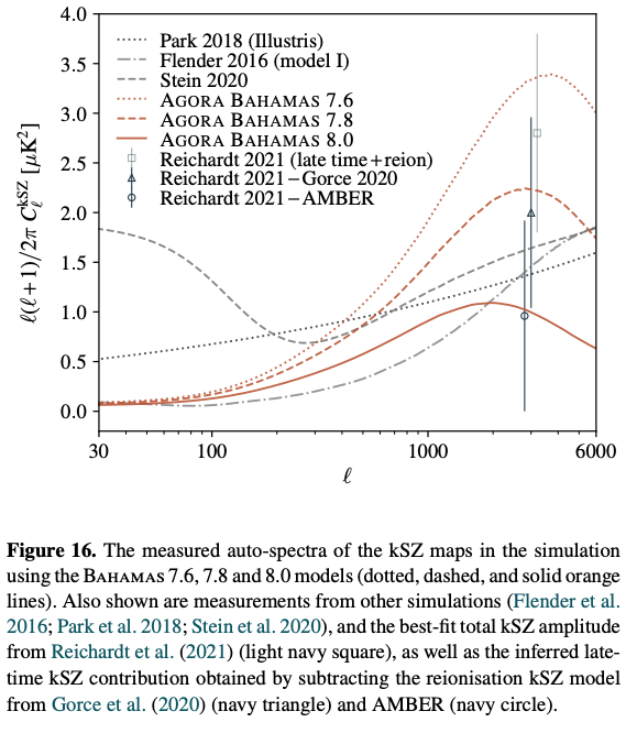
Note on kSZ Differences: The low-\(\ell\) excess seen in the WebSky model is primarily due to the large-scale Doppler term (bulk flow). WebSky and Agora have significantly different simulation box sizes; WebSky’s larger volume allows it to capture these large-scale bulk motions more effectively than Agora. Importantly, the high-\(\ell\) behavior—which is dominated by the small-scale kinematic effect—remains (substantially) consistent between the models. As shown in Agora Figure 16 (below), current empirical constraints from data are at very high \(\ell\) and carry large uncertainties.

fig, ax = plt.subplots(figsize=(6, 5))
for model in ksz_models:
    # Maps are in uK_CMB
    cls = hp.anafast(ksz_maps[model][0].value, lmax=lmax)
    d_ell = d_ell_factor * cls
    ax.semilogx(
        ells[1:],
        d_ell[1:],
        color=ksz_colors[model],
        label=ksz_titles[model],
    )

ax.set_title(f"kSZ Power Spectrum at {ksz_freq} GHz")
ax.set_xlabel("$\\ell$")
ax.set_ylabel("$\\ell(\\ell+1)C_\\ell / 2\\pi$ [$\\mu K^2$]")
ax.grid(True, which="both", alpha=0.3)
ax.legend(loc="lower left")
ax.set_ylim(0, 2.6)
fig.tight_layout()
fig.savefig("ksz_power_spectrum.png")

# Create composite plots for report
import matplotlib.image as mpimg

fig_tsz, axes_tsz = plt.subplots(1, 2, figsize=(12, 5))
axes_tsz[0].imshow(mpimg.imread("tsz_power_spectrum.png"))
axes_tsz[0].axis("off")
axes_tsz[0].set_title("PySM tSZ Power Spectrum")
axes_tsz[1].imshow(mpimg.imread("figure5.png"))
axes_tsz[1].axis("off")
axes_tsz[1].set_title("WebSky Figure 5 (Reference)")
plt.tight_layout()
plt.savefig("tsz_composite.png")
plt.show()

fig_ksz, axes_ksz = plt.subplots(1, 3, figsize=(18, 5))
axes_ksz[0].imshow(mpimg.imread("ksz_power_spectrum.png"))
axes_ksz[0].axis("off")
axes_ksz[0].set_title("PySM kSZ Power Spectrum")
axes_ksz[1].imshow(mpimg.imread("figure6.png"))
axes_ksz[1].axis("off")
axes_ksz[1].set_title("WebSky Figure 6 (Reference)")
axes_ksz[2].imshow(mpimg.imread("figure16.png"))
axes_ksz[2].axis("off")
axes_ksz[2].set_title("Agora Figure 16 (Reference)")
plt.tight_layout()
plt.savefig("ksz_composite.png")
plt.show()